UPDATE no. 2: Implementation Guide: SUM values if font is bold – Google Drive Spreadsheet

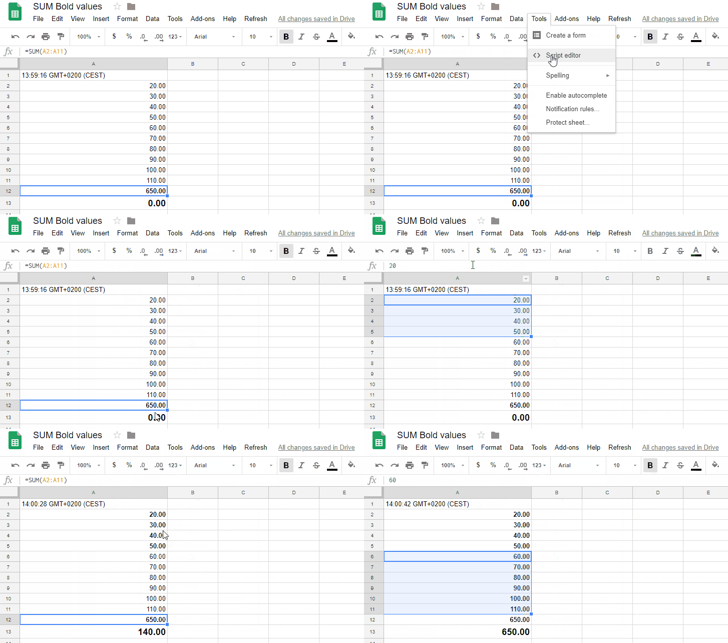
NEW: Screen recording of the solution at the end of this post.

This is the second part of the guide on how to implement custom functions into Google Drive Spreadsheets.

UPDATE: If you would like to easily update calculated values from this custom function than you have to go the following way: http://stackoverflow.com/questions/17341399/refresh-data-retrieved-by-a-custom-function-in-google-spreadsheet – I just followed mentioned guide there and I have an extra button in the menu now, which allows me easily refresh all values which were calculated by my custom function.

I have been receiving many questions about how exactly to use the script mentioned in the previous part of this guide so I decided, that it would be better to write it down incl. screenshots.

1. Open some of Your already created spreadsheets or create a blank one

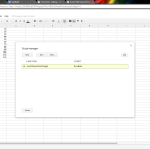
2. Using the main menu at the top choose: Tools -> Script manager

3. In this dialog click the New button and it will guide You to the Scripts editor

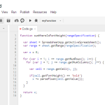
4. Paste following code into the editor, give some name to the script (top left corner input field), and Save it (Ctrl+S)

function sumWhereIsFontWeight(rangeSpecification) {

var sheet = SpreadsheetApp.getActiveSpreadsheet();
var range = sheet.getRange(rangeSpecification);

var x = 0;

for (var i = 1; i <= range.getNumRows(); i++) {
for (var j = 1; j <= range.getNumColumns(); j++) {

var cell = range.getCell(i, j);

if(cell.getFontWeight() == 'bold')
x += parseFloat(cell.getValue());
}
}

return x;
}

4. Get back to spreadsheet window and reload Your Scrip Manager dialog (circle arrow icon in top right corner) and You should see Your newly created script

5. Now You should be able to use this function in Your spreadsheet. To make it more clear, I added to the A column demo of what I added into columns in the B column (of course without those slashes at the beginning “//”). Here is screenshot of demo: